Continuous Distributions

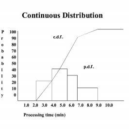
Continuous distributions are characterized by an infinite number of possible outcomes, together with the probability of observing a range of these outcomes. In the following example, there are an infinite number of possible operation times between the values 2.0 minutes and 8.0 minutes. Twenty percent of the time the operation will take from 2.0 to 3.5 minutes, 40% of the time the operation will take from 3.5 to 5.0 minutes, 30% of the time the operation will take from 5.0 to 6.0 minutes, and 10% of the time the operation will take from 6.0 minutes to 8.0 minutes.

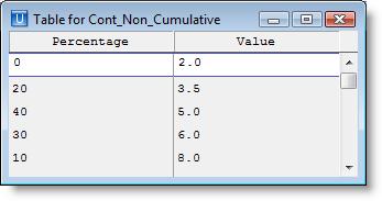
As with a discrete distribution, a continuous distribution can be defined in two ways. A probability density function lists each range of values along with the probability that an observed value will fall within that range. Each of the values within the range has an equal chance of being observed, hence the piece-wise linearity of the c.d.f. within each range of values. A probability density function for the example above is expressed as follows.

P(0.0 <= X < 2.0) = 0.00
P(2.0 <= X < 3.5) = 0.20
P(3.5 <= X < 5.0) = 0.40
P(5.0 <= X < 6.0) = 0.30
P(6.0 <= X <= 8.0) = 0.10
P(8.0 < X) = 0.00

The following table represents the p.d.f. for this example.

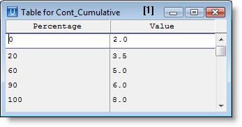
As with a discrete distribution, a cumulative distribution function for a continuous distribution specifies the probability that an observed value will be less than or equal to a specified value. A c.d.f. for the example distribution is as follows (where x represents the return value).

x 2.0 3.5 5.0 6.0 8.0

P(X <= x) 0 .20 .60 .90 1.0

The following table represents this c.d.f.